5  Trajectory with wind

In this second chapter of the advanced tutorial, we will see how to model the trajectory of the Great Reed Warbler using wind data.

Wind can significantly influence a bird’s movement, explaining up to 50% of the displacement! Accounting for wind allows to estimate the airspeed of each transition rather than groundspeed. As such, the movement model can be defined as the probability of a bird’s airspeed, which is much more constrained and precise. This approach is presented in detail in section 2.2.4 of Nussbaumer et al. (2023).

5.1 Download wind data

Wind data is available at high resolution (1hr, 0.25°, 37 pressure level) on ERA5 hourly data on pressure levels (Copernicus Climate Change Service 2018). This data is easily accessible through the ecmwfr package.

The first step is to set up your CDS access. You will need to create an account on cds.climate.copernicus.eu to generate your API key and uid number. You can store them as environment variables in your .Renviron using usethis::edit_r_environ().

cds_key = "Insert_your_CDS_API_KEY_here"
cds_user = "Insert_your_CDS_UID_here"

As the flights tend to be of short duration, we suggest downloading a file for each flight. This can be done automatically with tag_download_wind(), which uses wf_request_batch() to make all the requests in parallel.

tag_download_wind(tag)

You can monitor the requests at https://cds.climate.copernicus.eu/cdsapp#!/yourrequests. The files will be downloaded in data/wind/

In case you have a lot of tracks for which you need to download wind data and don’t want to block your console, you might consider using an RStudio background job, which can be easily called with the job package:

job::job({
  tag_download_wind(tag)
})

5.2 Create graph

Similar to the example of the Swainson’s Warbler in the basic tutorial, we first need to create the trellis graph:

graph <- graph_create(tag, quiet = TRUE)

5.3 Add wind to graph

We then compute the average windspeed experienced by the bird for each edge of the graph. This process can be quite long as we need to interpolate the position of the bird along its flight on a 4D grid (latitude-longitude-pressure level-time).

We then compute the airspeed based on this windspeed and the known groundspeed. All of these are stored as complex values with the real part representing the E-W component and the imaginary part corresponding to the N-S component.

graph <- graph_add_wind(graph, pressure = tag$pressure, quiet = TRUE)

5.4 Define movement model

While you can still define the movement model with a parametric function (i.e., gamma or logit), we find it more intuitive to use the mechanical power curve. The power curve expresses the energy required for a bird to fly at a certain airspeed based on aerodynamic theory. See more details in section 2.2.5 of Nussbaumer et al. (2023).

First, we search for morphological information on the Great Reed Warbler using the AVONET database (Tobias et al. 2022).

bird <- bird_create("Acrocephalus arundinaceus")

Using the bird created, we can set the movement model by converting the airspeed to power, and power to a probability. This second step is still a parametric equation, which can be manually defined with power2prob.

graph <- graph_set_movement(graph,
  method = "power",
  bird = bird,
  power2prob = \(power) (1 / power)^3,
  low_speed_fix = 15
)
plot_graph_movement(graph)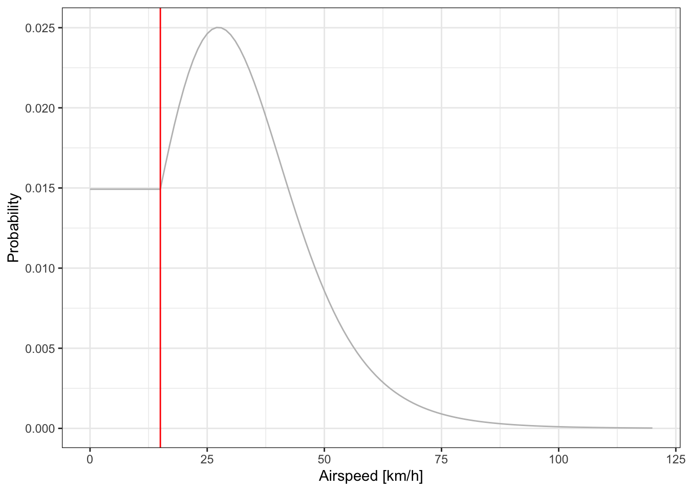

5.5 Products

We can then compute the same three products as for the Swainson’s Warbler:

path_most_likely <- graph_most_likely(graph, quiet = TRUE)
marginal <- graph_marginal(graph, quiet = TRUE)
path_simulation <- graph_simulation(graph, nj = 10, quiet = TRUE)

plot(marginal, path = path_most_likely)

plot_path(path_simulation, plot_leaflet = FALSE)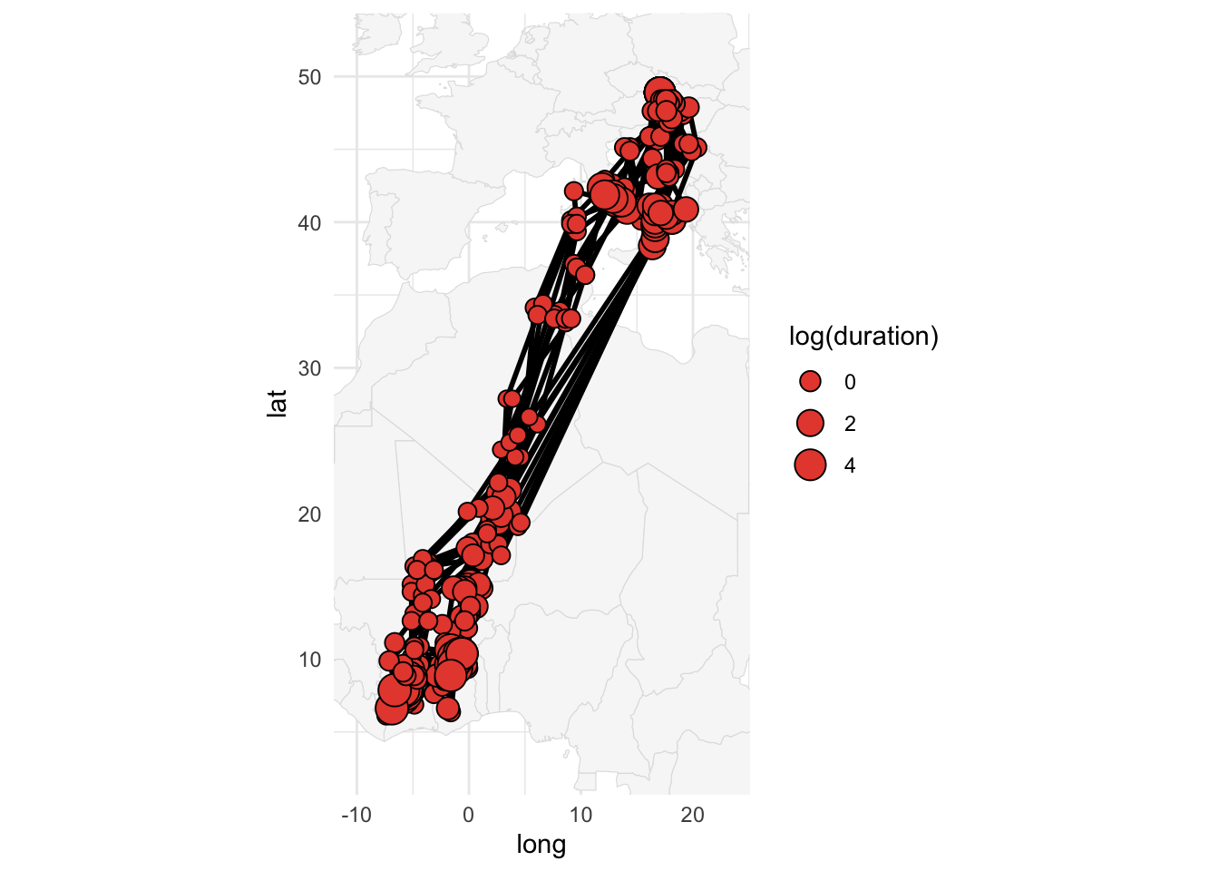

5.5.1 Extract flight information

The pathvariable contains all the information at the scale of the stationary period. However, to get flight information, you need to extract variable of the edge of the graph. path2edge() is the function for that!

edge_simulation <- path2edge(path_simulation, graph)
edge_most_likely <- path2edge(path_most_likely, graph)
knitr::kable(head(edge_most_likely, 3), digits = 1)

	stap_s	stap_t	s	t	lat_s	lat_t	lon_s	lon_t	start	end	duration	n	distance	bearing	gs	ws
1	1	2	26405	57010	48.9	47.6	17.0	16.4	2017-08-04 19:47:30	2017-08-04 23:17:30	3.5	1	150.4	-160.3	-14.2-34.8i	13.8-13.6i
12	2	3	57010	86621	47.6	44.9	16.4	14.4	2017-08-05 19:27:30	2017-08-06 02:52:30	7.4	1	342.4	-152.5	-20.2-38.7i	-5.5-4.6i
22	3	4	86621	118434	44.9	41.6	14.4	15.1	2017-08-06 19:12:30	2017-08-07 03:17:30	8.1	1	366.2	170.2	7.3-42.3i	-7.8-20.6i

edge_simulation$name <- glue::glue("{edge_simulation$stap_s}->{edge_simulation$stap_t}")
plot1 <- ggplot(edge_simulation, aes(reorder(name, stap_s), abs(gs))) +
  theme_bw() +
  ylab("gs") +
  geom_boxplot()
plot2 <- ggplot(edge_simulation, aes(reorder(name, stap_s), abs(ws))) +
  theme_bw() +
  ylab("ws") +
  geom_boxplot()
plot3 <- ggplot(edge_simulation, aes(reorder(name, stap_s), abs(gs - ws))) +
  theme_bw() +
  ylab("as") +
  geom_boxplot()
plot4 <- ggplot(edge_simulation, aes(reorder(name, stap_s), duration)) +
  theme_bw() +
  ylab("duration") +
  geom_point()

plotly::subplot(
  plotly::ggplotly(plot1),
  plotly::ggplotly(plot2),
  plotly::ggplotly(plot3),
  plotly::ggplotly(plot4),
  nrows = 4, titleY = TRUE
)

It’s a good idea to check the distribution of ground speed (gs), winspeed (ws) and airspeed (as) and check for any outliers which might come from error in the labeling. Here you can see the high groundspeed (>100km/h between stap 24 and 25) which is nicely explained by wind, as the corresponding airspeed is perfectly normal (~50km/h)

We can (and should) also check that our movement model is coherent with the distribution of flight speed assumed in the movement model:

plot_graph_movement(graph) +
  geom_histogram(
    data = data.frame(as = abs(edge_simulation$gs - edge_simulation$ws)),
    aes(x = as, y = after_stat(count) / sum(after_stat(count))),
    color = "black", fill = NA, bins = 100
  )

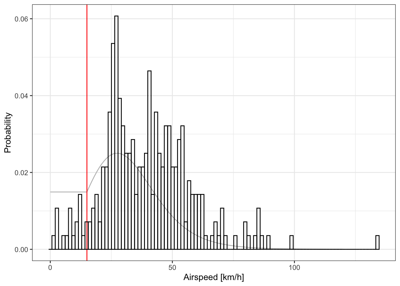
If you find anomalous flight speed, it might be worth checking if this/these flight(s) have been correctly labelled.

5.6 Save

graph can become extremely big for such models and it might not be recommended to save it. Check its size with format(object.size(graph), units = "MB").

save(
  tag,
  graph,
  path_most_likely,
  path_simulation,
  marginal,
  edge_simulation,
  edge_most_likely,
  file = "./data/interim/18LX.RData"
)

Copernicus Climate Change Service. 2018. “ERA5 Hourly Data on Pressure Levels from 1940 to Present.” Copernicus Climate Change Service (C3S) Climate Data Store (CDS). https://doi.org/10.24381/CDS.BD0915C6.

Nussbaumer, Raphaël, Mathieu Gravey, Martins Briedis, Felix Liechti, and Daniel Sheldon. 2023. “Reconstructing bird trajectories from pressure and wind data using a highly optimized hidden Markov model.” Methods in Ecology and Evolution 2023 (February): 1–12. https://doi.org/10.1111/2041-210X.14082.

Tobias, Joseph A., Catherine Sheard, Alex L. Pigot, Adam J. M. Devenish, Jingyi Yang, Ferran Sayol, Montague H. C. Neate-Clegg, et al. 2022. “AVONET: Morphological, Ecological and Geographical Data for All Birds.” Edited by Tim Coulson. Ecology Letters 25 (3): 581–97. https://doi.org/10.1111/ele.13898.