6  Pressurepath

In this chapter, we will see what a pressurepath object is and how to use it to compute the altitude of the bird throughout its trajectory.

Let’s load the tag from the Great Reed Warbler (18LX) created in the advanced tutorial.

load("./data/interim/18LX.Rdata")

6.1 Timeseries at a single position

Before creating a full pressurepath, we start with the basic building block of a pressurepath, which is to retrieve the pressure timeseries from ERA5 at a single location with geopressure_timeseries.

geopressure_timeseries relies on the pressure timeseries entry point of GeoPressureAPI which return the timeseries of pressure at a given latitude and longitude.

Let’s start by retrieving the pressure at the known site of equipment, querying the same date as the first stationary period.

ts <- geopressure_timeseries(
  lat = tag$stap$known_lat[1],
  lon = tag$stap$known_lon[1],
  start_time = tag$stap$start[1],
  end_time = tag$stap$end[1],
  quiet = TRUE
)

We can compare the retrieved ERA5 pressure to the pressure measured on the Great Reed Warbler:

p <- ggplot() +
  geom_line(data = ts, aes(x = date, y = surface_pressure, colour = "ERA5")) +
  geom_line(data = tag$pressure[tag$pressure$stap_id == 1, ], aes(x = date, y = value, colour = "tag")) +
  theme_bw() +
  ylab("Pressure (hPa)") +
  scale_color_manual(values = c("ERA5" = "black", "tag" = "red"))
layout(ggplotly(p), legend = list(orientation = "h"))

Eureka!

This was the figure that made me realize the potential of pressure measurement to determine birds’ position! The accuracy of the reanalysis data and the precision of the sensor were such that a timeseries of pressure had only a few possible options on the map.

6.2 Pressurepath

What is a pressurepath?

You can think of a pressurepath as the timeseries of pressure that a tag would record on a bird traveling along a specified path. To do that, pressurepath_create() calls geopressure_timeseries() for each stationary period and combines the resulting timeseries of ERA5 pressure.

The pressurepath data.frame returned also contains the original pressure pressure_tag which can be very helpful for labelling and the altitude of the bird corrected for the natural variation of pressure.

pressurepath <- pressurepath_create(
  tag,
  path = path_most_likely,
  quiet = TRUE
)

Note that if a position on the path is over water, it is automatically moved to the closest point onshore as we use ERA5 Land.

plot_pressurepath(pressurepath)

6.3 Altitude above sea level

The main benefit of creating pressurepath is the ability to retrieve ERA5 variable along the the trajectory of the bird. One of them is altitude which can be directly plot with

plot_pressurepath(pressurepath, type = "altitude")

Why use GeoPressureAPI for altitude?

Computing the bird altitude \(z_{gl}\) from its pressure measurement \(P_{gl}\) is best performed with the barometric equation

\[ z_{gl}=z_0 + \frac{T_0}{L_b} \left( \frac{P_{gl}}{P_0} \right) ^{\frac{RL_b}{g M}-1},\]

where \(L_b\) is the standard temperature lapse rate, \(R\) is the universal gas constant, \(g\) is the gravity constant and \(M\) is the molar mass of air.

It is typical to assume a standard atmosphere with fixed \(T_0=15°C\), \(P_0=1013.25 hPa\) and \(z_0=0 m\),

Lb <- -0.0065
R <- 8.31432
g0 <- 9.80665
M <- 0.0289644
T0 <- 273.15 + 15
P0 <- 1013.25
pressurepath$altitude_uncorrected <- T0 / Lb * ((pressurepath$pressure_tag / P0)^(-R * Lb / g0 / M) - 1)

However, we know that pressure and temperature vary considerably over time and space, leading to approximation in the altitude estimated.

Using GeoPressureAPI, we can adjust the barometric equation with the actual ground-level pressure \(P_{ERA}\) and ground temperature \(T_{ERA}\) retrieved from ERA5 at the bird’s location \(x\), \[ z_{gl}(x)=z_{ERA5}(x) + \frac{T_{ERA5}(x)}{L_b} \left( \frac{P_{gl}}{P_{ERA5}(x)} \right) ^{\frac{RL_b}{g M}-1},\]

See more information on the GeoPressureAPI documentation.

We can compare these two altitudes for the first stationary period,

The uncorrected altitude estimate incorrectly produces a 200m amplitude error in the altitude due to the natural variation of pressure. In contrast, the corrected altitude shows that the Great Reed Warbler mostly stayed at the same location/altitude during the entire period.

6.4 Altitude above ground level

In order to estimate the flight altitude above ground level, we need to retrieve the ground level elevation along the path. This can be done with path2elevation().

elevation <- path2elevation(path_most_likely,
  scale = tag$param$tag_set_map$scale,
  sampling_scale = tag$param$tag_set_map$scale * 2,
  percentile = c(10, 50, 90)
)

Note that because of the imprecision of the position, particularly during flight, it’s important to analyse with caution the relationship between flight altitude and ground elevation. path2elevation() aggregate the elevation across a larger area defined by scale and return different percentile.

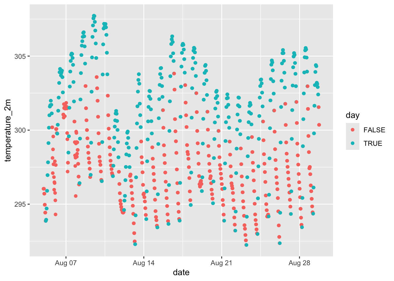
6.5 Retrieve ERA5 variables and sunrise along path

pressurepath_create() can also be used to retrieve other ERA5 variables along a path, such as temperature, cloud cover, and precipitation. This retrieve data from both ERA5-single-levels and ERA5-LAND dataset. Use GeoPressureR:::pressurepath_variable to list all the variables available. In addition, pressurepath_create() also computes the local sunrise and sunset time along the path using path2twilight().

pressurepath_2_to_5 <- pressurepath_create(
  tag,
  # in this example we only retrieve these variable between stationary period 2 and 5
  path = path_most_likely[path_most_likely$stap_id >= 2 & path_most_likely$stap_id <= 5, ],
  variable = c("altitude", "surface_pressure", "temperature_2m", "total_cloud_cover", "total_precipitation", "land_sea_mask"),
  solar_dep = -6,
  quiet = TRUE
)

6.6 Save

save(
  tag,
  graph,
  path_most_likely,
  path_simulation,
  marginal,
  edge_simulation,
  edge_most_likely,
  pressurepath,
  file = "./data/interim/18LX.RData"
)