1 Tag object
In this basic tutorial, we go through the main steps of GeoPressureR using only pressure data, with the example of a Swainson’s Warbler. This bird presents a short migration route, with only a few stopovers, making it easy to process and fast to compute.
1.1 Create tag
tag object?
A tag is a specific geolocator or datalogger which can contain multiple sensors (e.g., pressure, light, acceleration). Because such archival tag are usually not re-equipped, we consider that it is associated with a single deployment.
In GeoPressureR, tag is an object (i.e., a S3 class) which is created with the raw logger data. It is modified at each step of the workflow as it aggregates all the information needed to ultimately be able to model the bird’s trajectory.
The tag object is created based on the available data stored in ./data/raw-tag/CB619/ following the default structure described in GeoPressureTemplate.
tag <- tag_create(id = "CB619")✔ Read './data/raw-tag/CB619/CB619.deg'
✔ Read './data/raw-tag/CB619/CB619.deg'You can use the generic print() and plot() function to visualize the tag data.
plot(tag, type = "pressure")Depending on when you equipped the bird and when your tag started recording data, you likely need to crop your data to specific dates. As it is bad practice to modify your raw data, we recommend using the crop_start and crop_end arguments in tag_create().
1.2 Label tag into stationary periods
Labelling tracks involves two steps:
- Label periods of flight, which, by extension will define the stationary periods (called
stapin the code), during which the bird is assumed to remain at the same location (+/- tens of kilometres) and same elevation level (+/- few metres) - Discard pressure measurements which should not be used to estimate position (due to, for example, sensor error, flight, minor/short changes in elevation level, etc.)
Correctly labelling the track requires time and effort, but is key to accurately estimate the bird’s position.
As labelling relies on functions and tools presented later in the tutorial, we recommend first following the basic and advanced tutorials. After that, we strongly advise that you read attentively the recommendations for this step provided in Labelling tracks.
1.2.1 Initialize and create the label .csv file
Use tag_label_write() to initiate the label (i.e., empty label) and create the label file to ./data/tag-label/CB619.csv.
tag_label_write(tag)ℹ No label data.→ Initialize automatically label using `tag_label_auto()`✔ './data/tag-label/CB619.csv' written successfully.1.2.2 Label manually on Trainset
Open https://trainset.raphaelnussbaumer.com/ and click on “Upload Tag Label” to load your .csv file. Instructions on how to label the file can be found in the dedicated chapter Labelling tracks. Once you have finished, export the new csv file in the same folder /data/tag-label/CB619-labeled.csv (TRAINSET will automatically add -labeled in the name).
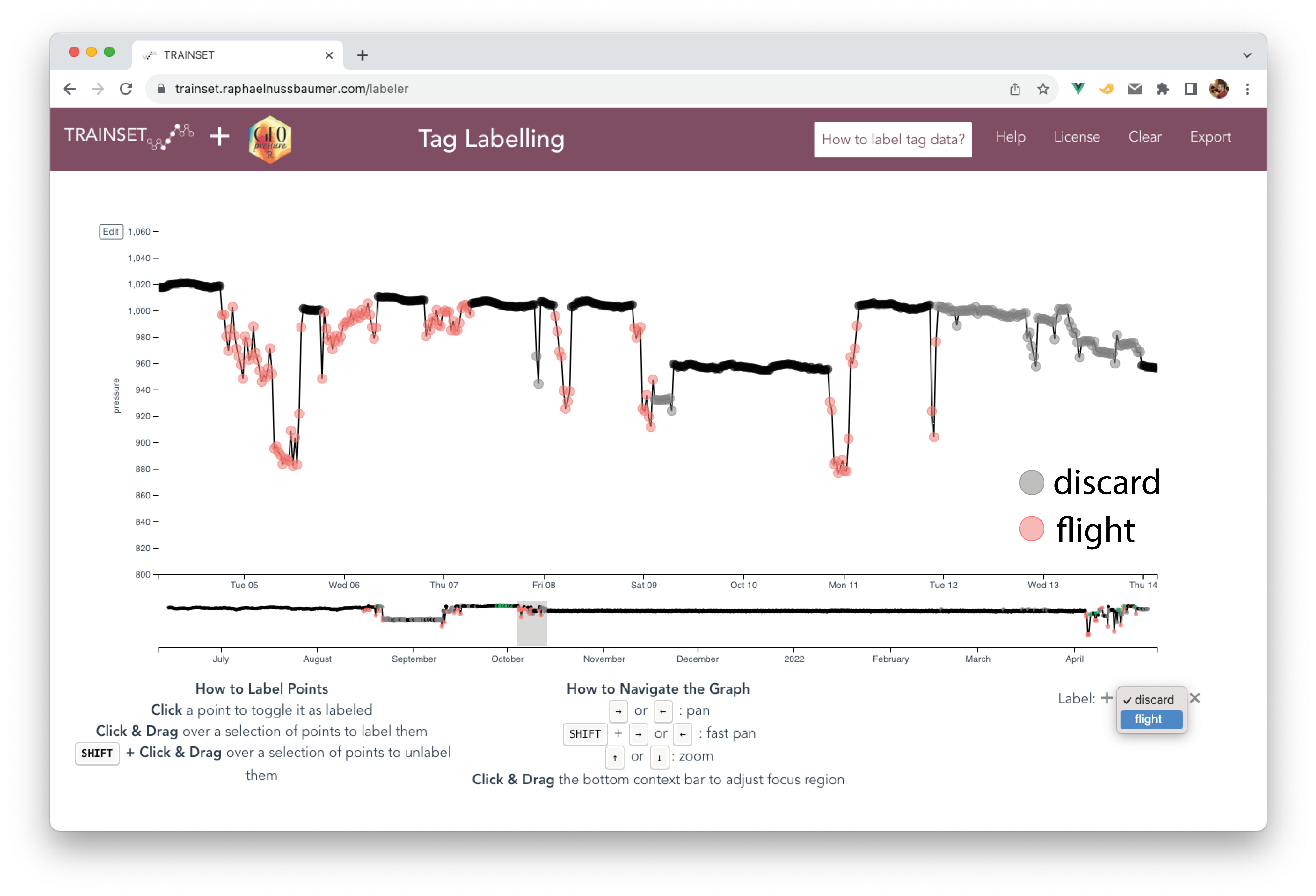
1.2.3 Read labelled file
Read the exported file with tag_label_read() to update tag$pressure (and, when relevant, tag$acceleration), with a new label column.
tag <- tag_label_read(tag)
knitr::kable(head(tag$pressure))| date | value | label |
|---|---|---|
| 2021-07-01 02:30:10 | 954.2268 | |
| 2021-07-01 03:00:10 | 954.0889 | |
| 2021-07-01 03:30:10 | 953.8978 | |
| 2021-07-01 04:00:10 | 953.6862 | |
| 2021-07-01 04:30:10 | 953.4887 | |
| 2021-07-01 05:00:10 | 953.0179 |
1.2.4 Compute stationary periods
tag_label_stap() then creates the stationary periods based on these labels:
tag <- tag_label_stap(tag, quiet = TRUE)
knitr::kable(head(tag$stap))| stap_id | start | end |
|---|---|---|
| 1 | 2021-07-01 02:30:10 | 2021-09-24 00:15:10 |
| 2 | 2021-09-24 11:15:10 | 2021-09-24 23:45:10 |
| 3 | 2021-09-25 10:45:10 | 2021-09-25 23:45:10 |
| 4 | 2021-09-26 12:45:10 | 2021-09-27 04:15:10 |
| 5 | 2021-09-27 08:15:10 | 2022-04-06 00:45:10 |
| 6 | 2022-04-06 10:15:10 | 2022-04-07 00:15:10 |
Plotting the pressure timeseries of tag provides additional information:
plot(tag, type = "pressure")You might notice some discrepancies between the raw data (grey) and the pre-processed pressure timeseries of each stationary period (colored lines).
The pre-processing aligns the raw timeseries data to the weather reanalysis pressure data by removing outliers and downscaling the resolution to 1hr falling on the exact hour.
The black dots show the discarded pressure points (i.e., outliers), corresponding to bird vertical movement rather than natural variation of pressure.
The function tag_label() is a wrapper for tag_label_write(), tag_label_read() and tag_label_stap(), allowing you to process the label file (i.e., CB619-labeled.csv) in a single line.